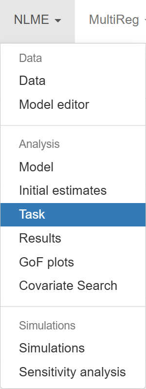
Task
The "Task" section provides tools to initialize and manage the statistical components used during the model calibration process.
Work in this tab begins by clicking the  button. This sets the path to a folder where the configuration of statistical components and the results of model fitting will be stored.
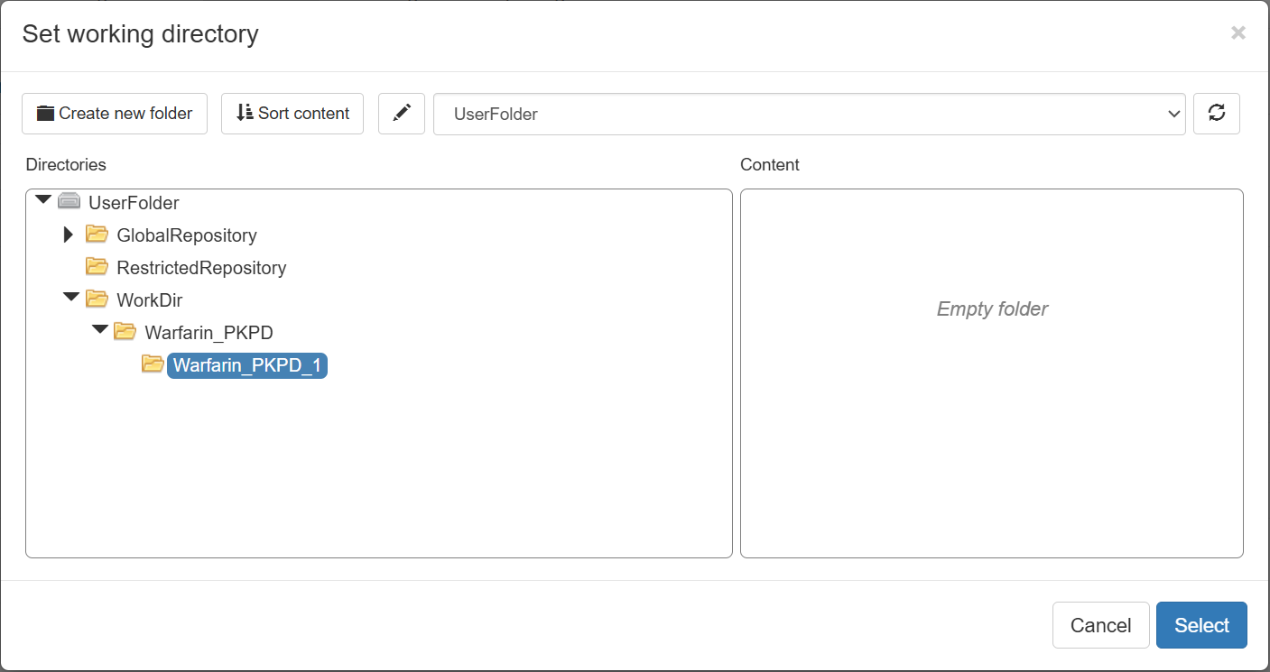
You may select either a new (empty folder) directory or one that contains results from a previous fitting session. If the directory already contains results, you can skip earlier steps (e.g., Data, Model, or Initial estimates) and move directly to task section.
After selecting the working directory, four main options become available:
-
 loads previously saved fitting results from the selected directory. Once loaded, you can proceed to tabs like Results, GoF plots, or Simulations to evaluate or utilize the fitted model.
 -
 loads a previously saved configuration of the statistical components. After loading, select the fitting algorithm (e.g., Simurg, Monolix, or nlmixr) and proceed to
  .
. -
 cleans the directory if it contains files and opens a list of options for configuring the statistical components. This option requires that the Data, Model (or Model editor), and Initial estimates tabs have already been properly initialized.
 -
 deletes all contents from the selected directory, allowing you to start fresh with a new statistical component configuration.
Creating statistical model
The process of creating a statistical model in the "Task" tab is divided into four key components:
1. Residual error model
In pharmacometric modeling, the residual error model captures the unexplained differences between observed data and model predictions — those not accounted for by the structural model or inter-individual variability.
Simurg offers several residual error model options for each specified DVID, including:
-
Constant error (independent of the predicted value): $$ y = f + \epsilon, \epsilon ∼ N(0, a^2)$$
-
Proportional error (increases proportionally with the predicted value): $$ y = f \cdot (1 + \epsilon), \epsilon ∼ N(0, b^2)$$
-
Combined1 error (constant + proportional): $$ y = f + \epsilon, \epsilon ∼ N(0, a^2 + (b·f)^2)$$
Here, \(f \) is the predicted value, and \( a \) and \( b \) are estimated error parameters.
The fields for selecting the residual error model and its parameters look like this:
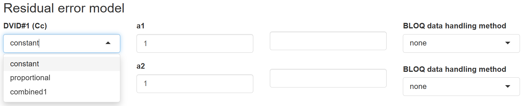
Additionally, you can specify how BLOQ (Below Limit of Quantification) data are handled. Available methods include:
- M3: BLOQ data points are treated as left-censored values.
- M4: A hybrid method where:
- BLOQ values before the first quantifiable observation are treated as censored
- BLOQ values after are treated as missing (ignored)
These options are only available if your dataset (initialized in the Data tab) contains the required columns:
- For M3:
CENS - For M4:
CENSandLIMIT
If these columns are not present, the default handling method is "none".
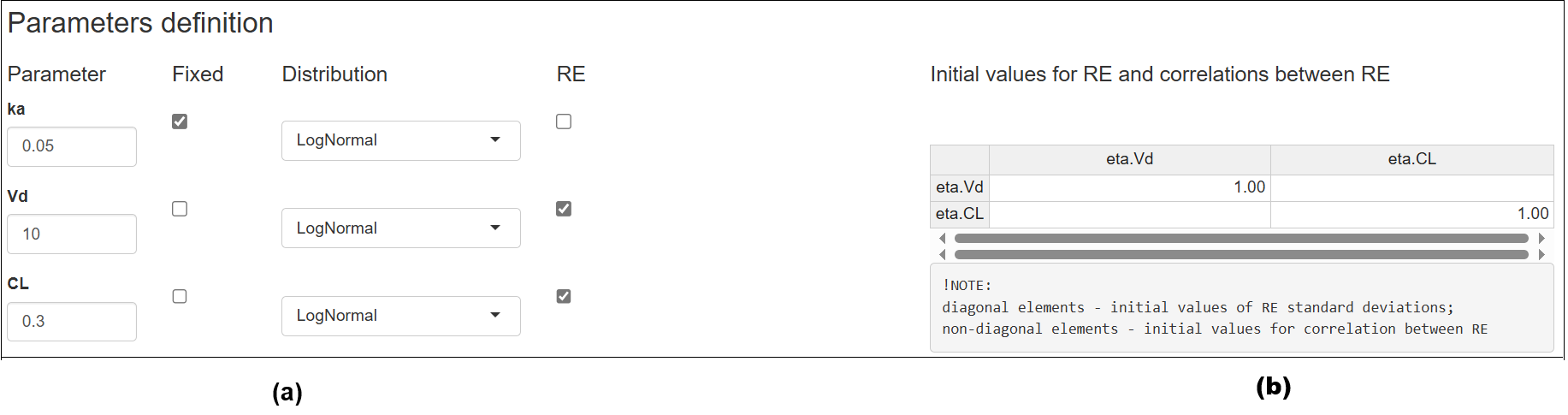
2. Parameter definition
This section allows you to define the characteristics of model parameters during the fitting process (Figure 1(a)). Specifically, you can determine:
-
Whether a parameter is fixed or includes random effects
-
The distribution type used to model the random effects
📌 Note: The distribution settings apply to random effects, not the fixed effect estimates themselves.
Available distributions in Simurg include:
| Distribution | Formula |
|---|---|
| Normal | \( P_i=\theta +\eta_i, \space\space \eta ∼ N(0,\omega^2)\) |
| Lognormal | \( P_i=\theta + \exp(\eta_i), \space\space \eta ∼ N(0,\omega^2)\) |
| Logit-normal | \( P_i=\frac{1}{1+\exp(-(\theta+\eta_i))}, \space\space \eta ∼ N(0,\omega^2)\) |
where \(\theta\) is the typical value of a parameter, \(\eta_i\) the random effect for individual \(i\), and \(\omega\) is the standard deviation of \(\eta\).
In addition, you can specify initial values for random effects and their correlations using the matrix provided on the right-hand side of the interface (Figure 1(b)). This matrix allows for the configuration of:
- Variances – Initial guesses for \(\omega^2\), representing the variability of each random effect.
- Correlations – Initial values for the correlations between random effects (typically set to 0 unless prior knowledge suggests otherwise).
Matrix structure:
- Diagonal elements represent the initial values for the standard deviations of the random effects (i.e., \(\omega^2\)).
- Off-diagonal elements define the initial correlations between the corresponding random effects.
These initial values can influence the convergence behavior of the fitting algorithm, so it's recommended to use reasonable estimates when available.
3. Covariate model
This section allows you to introduce covariate effects into the model, enabling more personalized and accurate parameter estimation based on individual-specific characteristics from the dataset.
The interface looks like this:
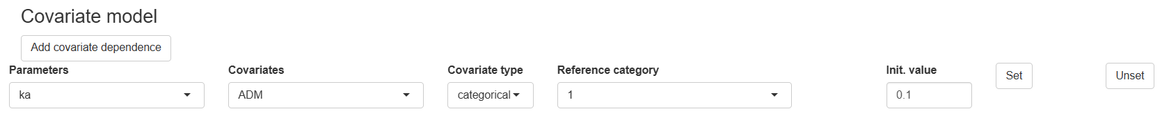
To add a covariate effect:
1. Select the parameter you want the covariate to influence.
2. Choose the covariate from the list (the name must match a column in the initialized dataset).
3. Specify the covariate type:
-
Categorical: Define the reference category, which serves as the baseline level for comparison.
-
Continuous: Choose both a function to describe the covariate relationship and a central tendency transformation (mean or median) to normalize the covariate.
Functions for Continuous Covariates
Simurg provides several functional forms to model continuous covariate relationships:
- Linear (lin): $$\theta_i = \theta_{ref} \cdot (1+\beta \cdot (x_i-x_{ref}))$$ A direct linear relationship between the covariate and the parameter.
- Log-linear (loglin): $$\theta_i = \theta_{ref} \cdot \exp(\beta \cdot (x_i-x_{ref}))$$ A multiplicative effect, useful when the effect increases or decreases exponentially.
- Power model: $$\theta_i = \theta_{ref} \cdot \left( \frac{x_i}{x_{ref}} \right) ^\beta $$ A flexible model that can capture nonlinear proportional effects, often used in allometric scaling.
Where \(\theta_i\) is the individualized parameter estimate, \(\theta_{ref}\) is the parameter value at the reference covariate value \(x_{ref}\), \(\beta\) is the estimated covariate effect, \(x_{i}\) is the individual's covariate value.
You can choose whether \(x_{ref}\) is based on the mean or median value of the covariate in the dataset.
4. Specify the initial value for the parameter associated with the reference category (for categorical covariates) or the normalized value (for continuous covariates).
5. Click "Set" to apply the covariate effect to the selected parameter.
Once all configurations are complete, click the  button. This action saves the statistical model setup—defined in the previous sections to the selected working directory.
4. Optimization options
📌 Options in this section will become available only after the control object is created.
After the control object has been successfully created:
Select the fitting algorithm you wish to use (e.g., Simurg, Monolix, or nlmixr).
Click to begin the model fitting process.
When the fitting is complete, you can move on to the Results tab to analyze the output and evaluate the model's performance.