Results
Essential output of a model calibration procedure includes several numerical characteristics and scores, such as:
- point-estimates of population parameter values;
- standard deviation (SD) of random effects;
- eta-shrinkage;
- standard errors (SE) for all parameters;
- individual parameter values if random effects are present in the model;
- correlation between parameters;
- likelihood-based numerical criteria.
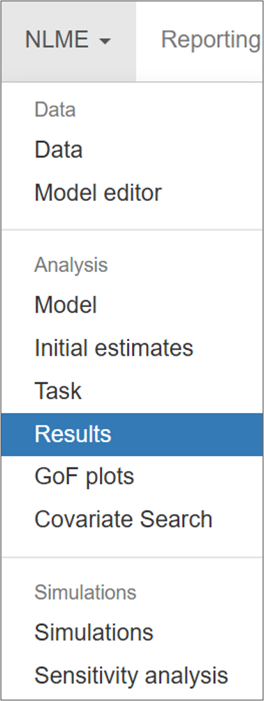
To extract this infromation from a modeling project, either a calibration procedure should be performed or the results of a calibration procedure should be loded following the instructions for the Task section. Once it is done, Results section in NLME can be accessed:
and relevant output can be generated by pressing  button.
Generated output is spread across four tabs:
After "View model results" button is pressed,  button will appear below it. By pressing this button all figures and tables from all four tabs will be saved to location of the current project within Simurg environment.
In addition,  button, available on the first 3 tabs, allows to export figures or tables from a tab to local computer.
1. Summary
Summary tab contains essential information in a form of a summary table on model parameters obtained after a calibration procedure:
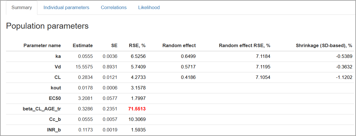
Parameter names are shown exactly as specified in the structural model.
Covariate coefficients are named using the following principle:
[parameter name]_[covariate name]_[transformation flag]
Residual error model parameters are assigned as follows:
[variable name]_[a - for additive component; b - for proportional component]
\(SE\) of the parameters are calculated in three steps.
First, variance-covariance matrix is calculated for transformed normally distributed parameters from the Fisher Information Matrix (FIM) as follows:
$$ C(\theta)=I(\theta)^{-1} $$
Next, \( C(\theta) \) is forward-transformed to \( C^{tr}(\theta) \) using the formulas to compute the variance, dependent on the distribution of the parameters:
- For normally distributed parameter: no transformation applied.
- For log-normally distributed parameters: $$ SE(\theta_k)=\sqrt{( \exp(\sigma^2)−1) \cdot \exp(2\mu + \sigma^2)} \\ \mu = \ln(\theta_k) \\ \sigma^2 = \operatorname{var} (\ln (\theta_k)) $$
- For logit-normally distributed parameters: a Monte Carlo sampling approach is used. \(100000\) samples are drawn from the covariance matrix in gaussian domain. Then the samples are transformed from gaussian to non-gaussian domain. Then the empirical variance \( \sigma^2 \) over all transformed samples \( \theta_k \) is calculated.
Finally, \(SE\) of the estimated parameter values is calculated from the diagonal elements of the forward-transformed variance-covariance matrix: $$ SE(\theta_k) = \sqrt{C^{tr}_{kk}(\theta_k)} $$
Relative standard error (\(RSE\)) is calculated as \( \frac{SE}{Estimate} \cdot 100 \% \).
Cases with \(RSE > 50 \% \) are highlighted in red, as \(RSE > 50 \% ( \frac{1}{1.96} * 100 \% ) \) corresponds to the situation where \( 95 \% \) confidence interval of \( N(0, 1) \) includes zero, making respective parameter not statistically different from zero with \( \operatorname{p-value} = 0.05 \).
Random effects column contains \(SD\) of the estimated random effects \( (\omega) \).
\( \eta \)-shrinkage is calculated based on the following equation: $$ \eta \space shrinkage = 1 - \frac{SD(\eta_i)}{\omega} $$ \( \eta \)-shrinkage exceeding \( 30 \% \) is indicative of unreliable individual parameter estimates and warrants the revision of a statistical model [1].
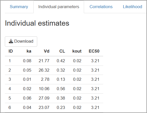
2. Individual parameters
This tab contains a single table with individual parameter values defined as the mean of conditional distribution for parameters with random effects and as typical parameter values for the parameters without random effects.
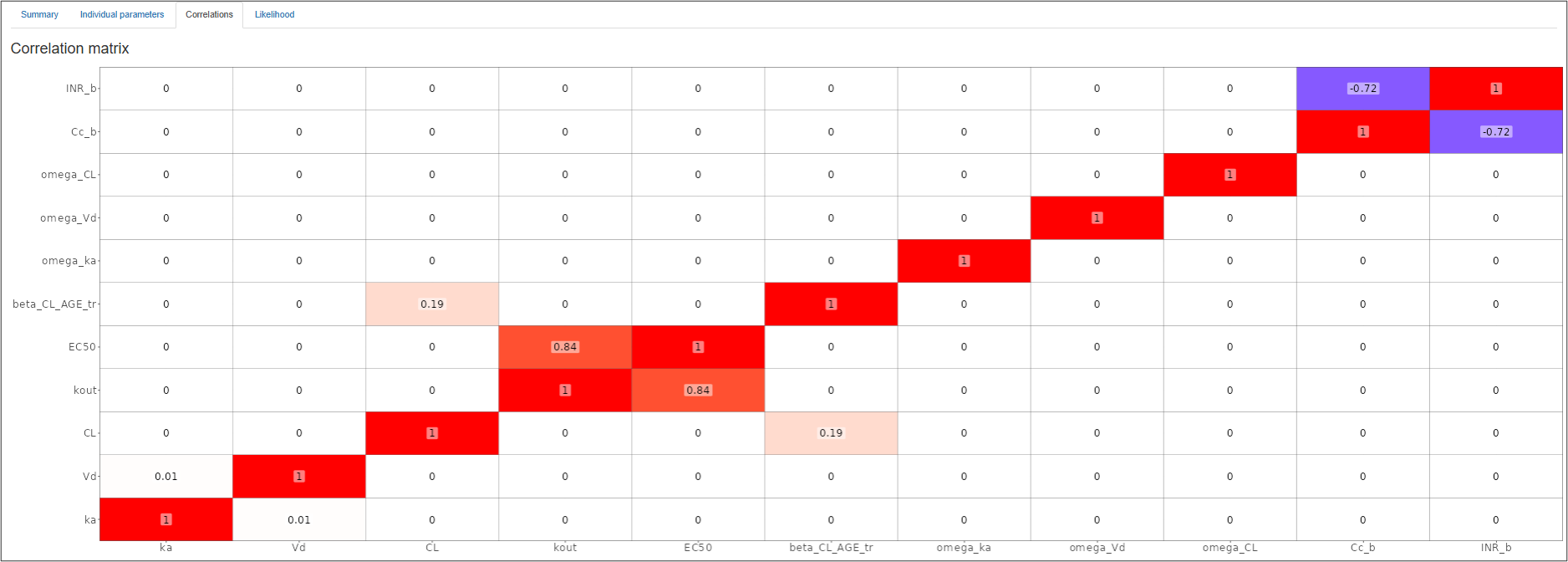
3. Correlations
Correlation matrix is derived from the variance-covariance matrix as:
$$ \operatorname{corr}(\theta_i, \theta_j) = \frac{C^{tr}_{ij}}{(SE(\theta_i)*SE(\theta_j))} $$
and is represented visually in a form of a heatmap, where the value and color in each cell represents Pearson's correlation coefficient (blue - for negative values, red - for positive values).
4. Likelihood
This tab contains likelihood-based numerical scores used to benchmark models:
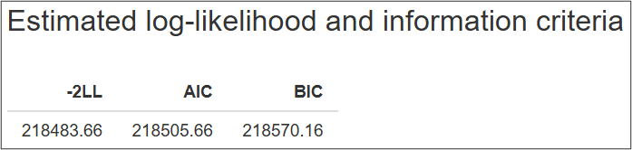
- \( -2 \cdot \log(\operatorname{Likelihood}): n \log(2\pi)+\sum(\log(\sigma_j^2 ) + \frac{(Y_j-Y^*_j (t,\Theta))^2}{\sigma_j^2}) \)
- Akaike information criterion: \( AIC = -2LL + 2 \cdot P \)
- Bayes information criterion: \( BIC = -2LL + P \cdot \log(N) \)
where \( P \) is the number of estimated parameters within the model; \(N \) is the number of data points.
N.B.: likelihood cannot be computed in a closed form if random effects are present in the model.
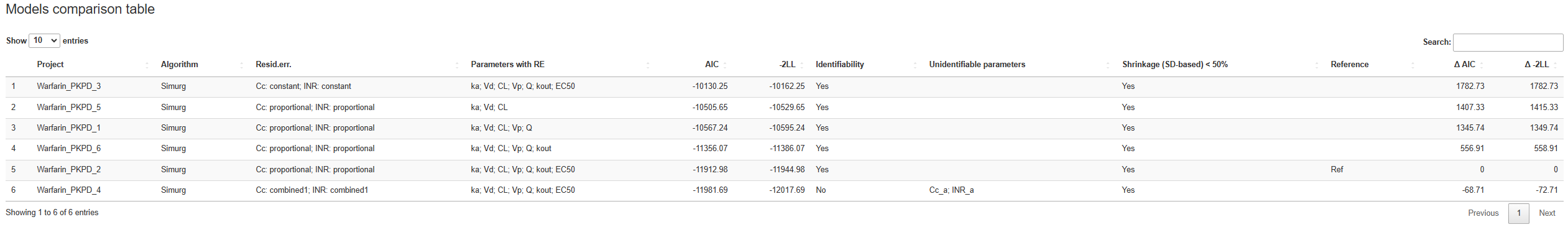
Model comparison
"Likelihood" tab allows to perform semi-automatic model comparison across multiple projects, located within the same folder of the currently active project by pressing  , selecting the subset of projects to include into the analysis (optional), and pressing
  button.
For example, running model comparison given the following folder structure:
parent-folderWarfarin_PKPD_1Warfarin_PKPD_2- current projectWarfarin_PKPD_3Warfarin_PKPD_4Warfarin_PKPD_5Warfarin_PKPD_6
where Warfarin_PKPD_1 ... Warfarin_PKPD_6 are successfully converged computational projects, will provide user with the following table:
By indicating character string in the  field, for example,
 project1, will leave only those projects in the table that contain this string within their names.