Forward Simulations
In this tab, users can perform and visualize simulations using one of the fitted models
There are two panels at this tab:
Simulation optionsallows users to configure simulation settingsVisualization optionsenables customization of the simulation visualization
Simulation options
Forward simulations represent the final step in the exposure-response (ER) analysis workflow. By this stage, it is assumed that the users have already completed all prior steps and have obtained a list of final models—one fitted model per clinical endpoint. This list is typically created during the covariate search step and saved as FinalModelsList.RData. Alternatively, the users may generate the list manually. In that case, the file must be named FinalModelsList.RData and formatted as a list of generalized linear models.
Selecting a Model for Simulations
To perform simulation, the users must first select the model they wish to use. This is done in two main steps within the interface:
-
Specify the Model Directory
The users must indicate the directory containing the model list. This is configured using the
Sourceinput, which provides two options:-
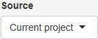 Uses the working directory selected in the Data Initialization panel.
 -
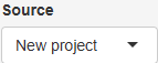 Allows users to specify a different folder by clicking
 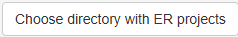 button
The path to the selected directory is displayed below the
Sourceinput, allowing the users to confirm the correct directory before proceeding.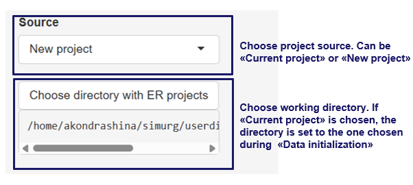
-
-
Load and Select the Model
Once the working directory is set, the users should clicks the  button to load the models from the
 FinalModelsList.RData into the interface.
After loading, the users select a specific model from the list by choosing its serial number via the 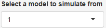 input. Once selected, the users can adjust covariate values within the interface and proceed to run simulations using the chosen model.
Adjusting Covariate Values for Simulations
This section explains how to change covariate values in the interface for simulations.
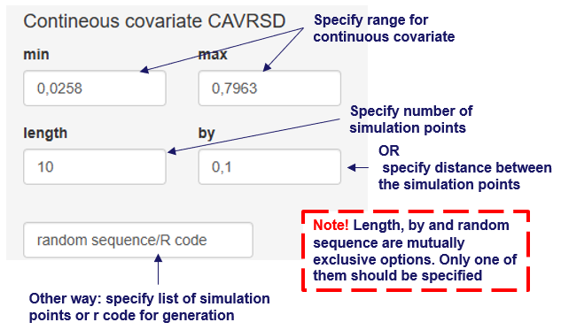
Continuous covariates
There are several ways to specify continuous covariates values to simulate with.
-
Define a range using
MinimumandMaximuminputs. Then, either:- Specify the number of points within this range using the
Lengthinput. - Define the interval between points using the
Byinput.
If
Lengthvalue is specified in the interface, theByvalue will be ignored. To useByvalue, clear theLengthinput. - Specify the number of points within this range using the
-
Enter a list of comma-separated covariate values into the
Random Sequenceinput. These values will be used for simulations. Note that this option works in the absence of theLengthandByvalues.
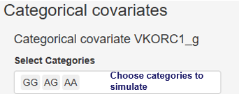
Categorical Covariates
Users can select specific values for categorical covariates to include in the simulation.
Selecting Output Type
Users can specify the Output Type for calculations, choosing between:
Response- the simulation results will be in response scales. For example, for binomial model the probability of response will be returned with this optionLink- the simulation results will be on the scale of linear predictors, without applying the link function. Currently this option is not available on the interfaceTerms- calculate a matrix giving fitted values in the model formula on the linear predictor scale. Currently it is not available on the interface
Confidence Intervals for Predictions
Users can toggle the inclusion of confidence intervals in model predictions using the  checkbox.
Running simulations
After configuring all simulation options, users must click the  button to start the process. The resulting plot can then be customized using the
 Visualization Options panel.
Visualization Options
In this panel, the user can customize how simulation results are displayed.
Main visualization options
The Select plot type input allows users to choose the type of plot. The available plot types are:
Scatterdisplays the simulated response versus the exposure metric as individual points. If standard errors (SE) were calculated on the Simulations panel, they will be shown as a ribbonPointrangesimilar to theScatterplot, but the SE is displayed as an interval around each point.Boxplotrepresents the simulated response using boxplots
Additional settings include:
Select X-axis variabledefines the variable to be used on the X-axisSelect color variablespecifies the variable used to color different data groupsSelect shape variableassigns different point shapes based on groupings defined by this variableSelect line type variabledetermines the line styles used for different groupsSelect group variabledefines the grouping variableSelect facet variablesets the variable used to split the data into facets (subplots)
Aggregation Options
To perform aggregation of simulation results, the users should specify the central tendency measure via the Select central tendency measure input. This input has three options:
Noneaggregation of the data will be doneMeanaggregation will be done by averaging the dataMedianmetric will be used for aggregation
Similarly, the variability can be selected by the Select variance measure with options:
SDstandard deviationRangemin-max rangeIQRinterquartile range80% CI80% confidence interval90% CI90% confidence interval95% CI95% confidence interval99% CI99% confidence interval
Plot Properties
If a Facet variable is defined, you can set the facet scaling using the Select facet scales input. Options include:
Free: both axes can vary across facetsFree_x: X-axis varies across facets; Y-axis remains fixedFree_y: Y-axis varies across facets; X-axis remains fixedFixed: Both axes remain the same across all facets
Other options:
Round X-values: specify the number of decimal places for X-axis ticks' labelsX as factor: check this box to treat X-axis values as categorical factorsAdd points: when enabled. observed data points will be added to boxplots
Cosmetics Settings
The title of the x axis can be customized by the X axis label input
Saving and Rendering Results
-
 button: click to render the plot using the current settings
 -
 button: saves the generated plot to the project directory. The name used to save the plot can be specified by
 Plot nameinput -
 button: saves the simulation results as a data table. The name used to save the simulation results can be specified by
 Table nameinput