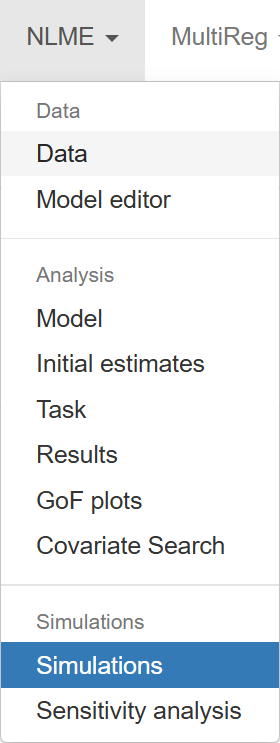
Simulations
The Simulations section enables users to simulate model predictions under various scenarios using either an already-fitted model or a new model file. It provides the tools necessary to set up simulation conditions, incorporate stochastic variability, adjust parameters, and generate results for visual inspection.
The simulation interface is organized into two main tabs, each with a set of clearly defined sections:
- Simulation
1.1. Simulation scenarios
1.2. Stochastic components
1.3. Parameters
1.4. Execution - Visualization
1. Simulation
Before configuring a simulation, you must first select the Source model.
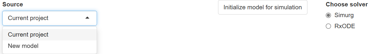
Two options are available:
-
Current project: Select this option if you want to simulate based on the model currently loaded and fitted in the project. Make sure that model fitting has been completed or previously saved results have been loaded, following the steps described in the Task section.
-
New model: Select this option if you wish to simulate using a different model not associated with the current project. In this case, the button
 will appear, allowing you to select a .txt file containing the model definition.
After selecting the source, choose the appropriate solver and click  to prepare the model for the simulation environment.
Once initialized, you can proceed to configure the remaining components of the simulation. These are divided into four sections:
1.1 Simulation scenarios
This section allows you to define the structure of your simulation by building or uploading an event table that outlines the dosing and observation scheme, along with any additional covariates. Simurg supports both Time profiles and Dose-response simulation types, offering flexibility for a wide range of simulation needs.
Simulation type
To begin, select the Simulation type to be performed:
-
Time profiles – to simulate concentration or response profiles over time.
-
Dose-response – to explore relationships between dose levels and outcomes.
You can either upload an existing event table, clicking  button, or manually create one using the built-in interface.
Creating an Event table manually
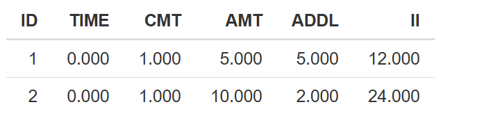
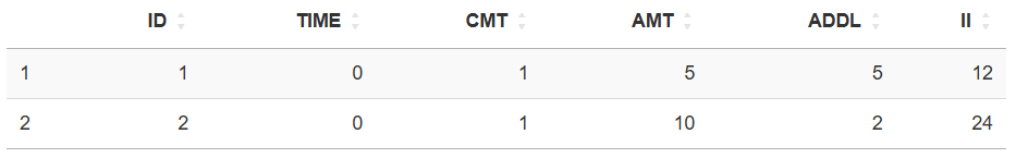
To manually create an event table, click the  button. This will generate a default event table with a new row corresponding to a unique ID (e.g., ID = 1, 2, 3…), representing each simulation scenario.
The default columns in the event table depend on the selected Simulation type:
-
For Time profiles:
ID: Identifier for each simulation scenario.TIME: Time points for dosing or observations.CMT: Compartment number.AMT: Administered dose amount.ADDL: Number of additional doses.II: Interdose interval (used with ADDL).
-
For Dose-response:
ID: Identifier for each scenario.TIME: Typically fixed or set to zero (if not time-based).CMT: Compartment number.MinDose/MaxDose: Minimum and maximum dose values for the simulated range.ADDLandII: Optional for repeated dose-response assessments.
You can click multiple times to define additional scenarios. Each click will append a new row to the table with the next available ID. To remove a scenario, use the  button.
Customizing columns The table can also be extended horizontally to include covariates or other input variables:
Enter a column name into the "New column name:" field.
Click  to add it to the table.
To remove the most recently added column, click  .
.
💡 Depending on your model, you may need to include additional columns beyond those added by default (e.g., covariates like WT, AGE, or SEX).
💡 When defining values directly in the event table, you can also assign fixed values to any system parameter used in the model. Once a variable is included in the event table, it will automatically be excluded from the "Parameters" section, and if the variable has an associated omega (random effect), it will not be included in the simulation. This allows you to override default parameter behavior with scenario-specific values when needed.
Editing the event table The event table is fully interactive: to modify a value, simply double-click on the desired cell and enter the new content. This makes it easy to adjust values on a scenario-by-scenario basis.
Time Grid and Output Settings
The final block in Simulation scenarios defines the temporal grid and the variables that will be returned by the solver.
| Setting | Purpose |
|---|---|
| Init. time | Start time of the simulation. |
| Min. time / Max. time | Left and right bounds of the time window forwarded to the Visualization tab. Any simulated points outside this interval are discarded. |
| Time step | Fixed increment between consecutive time points. |
| Vector length | Total number of nodes in the calculation grid. |
| Select output names | Choose the state variables or user-defined functions you wish to record. The items selected here populate Plotted outputs in the Visualization tab. If left blank, all available outputs are transferred automatically. |
📌 Note: You may define either the Vector length or the Time step, but not both. Setting Vector length to (0) (or leaving it blank) enables Time step input.
Additional Fields for Dose-Response Simulations When Simulation type is set to Dose-response, two additional configuration options become available in this section:
| Setting | Purpose |
|---|---|
| N of dosing steps | Specifies how many discrete doses will be evaluated between the defined MinDose and MaxDose values for each scenario. |
| Type of metrics | Determines the summary statistic to apply over the simulated time profile for each dose. Available options are:
|
1.2 Stochastic components
This subsection allows you to incorporate different levels of variability into the simulation, making it possible to generate more realistic outputs that reflect natural uncertainty in biological systems. Four building blocks are available; you may activate any combination, depending on the modeling objectives:
1.2.1. Use virtual populations
1.2.2. Add uncertainty
1.2.3. Add variability
1.2.4. Add residual error
1.2.1 Use virtual populations
Virtual populations (VPs) are computer-generated cohorts of virtual patients. Each virtual patient is a unique set of parameter and/or covariate values chosen to reflect realistic biological diversity. They allow you to run in silico trials without recruiting real volunteers.
After ticking Use virtual populations, several windows appear:
| Setting | Purpose |
|---|---|
| Number of virtual patients | Total VP size (10 by default). Each patient will be simulated once for every scenario in the event table. |
| Generate vs Upload VP | • Generate virtual population – create a fresh VP. • Upload virtual population – import a pre-built VP file ( .csv). Press “Choose file with VP” and the selected path is shown beneath the button. |
Generate virtual population
If Generate is chosen, two editable tables appear:
-
Select parameters or covariates
Tick the items you wish to vary. The chosen entries populate the Table of parameters distribution:
Distribution– choose LogNormal, Normal, or Uniform.Mean– central value (µ).SD– standard deviation (σ) for Normal / LogNormal.CV %– coefficient of variation (alternative to SD for LogNormal).Min/Max– bounds for Uniform (also used as hard limits for the other distributions).
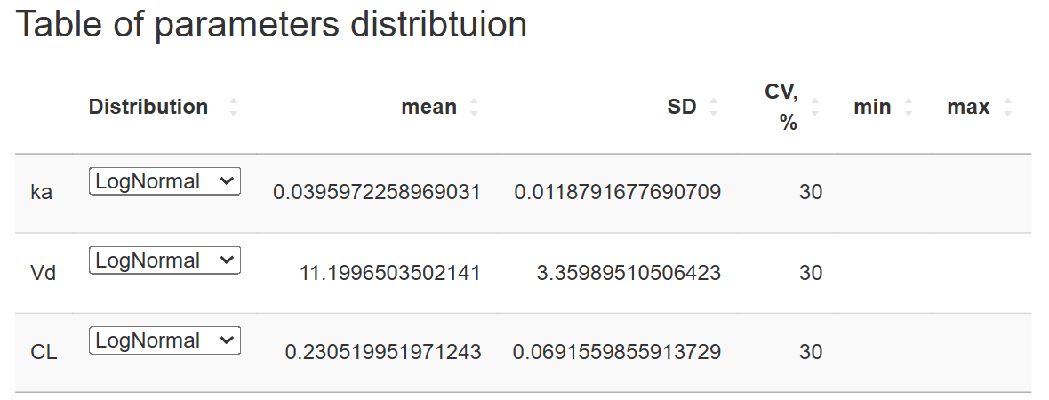
All cells are editable via double-click.
-
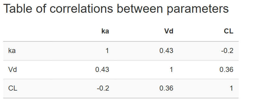
Table of correlations between parameters
A symmetric matrix whose diagonal is fixed at 1. Edit the lower-triangle cells to specify pairwise correlations (between [-1;1]); the upper-triangle mirrors automatically. Setting correlations helps reproduce realistic multivariate relationships.
After adjusting distributions and correlations, click  .
The VP is stored in memory (and can be exported later) and the remaining stochastic-component options become available.
.
The VP is stored in memory (and can be exported later) and the remaining stochastic-component options become available.
1.2.2 Add uncertainty Enables simulation of parameter uncertainty by resampling fixed effects from their estimated uncertainty distributions.
- Number of populations: Defines how many virtual populations will be generated by drawing parameter sets from the uncertainty distribution. Recommended: Start with at least 100 populations for stable results.
1.2.3 Add variability Introduces inter-individual variability by sampling random effects for each subject within each population.
- Number of subjects: Defines how many individuals will be simulated per population. Recommended: Use at least 20–50 subjects to capture population-level spread.
1.2.4 Add residual error Adds residual unexplained variability, typically representing measurement error or unmodeled intra-individual fluctuations.
- Number of replicates: Determines how many repeated observations will be simulated per individual at each time point. Recommended: Use 5–10 replicates for exploring variability bands around predicted profiles.
Each of these components adds a layer of realism to the simulation by mimicking the kinds of uncertainty and variability typically observed in PK/PD or QSP models. You can enable them individually or in combination to suit your analysis needs.
1.3 Parameters
This section is automatically populated once the model has been initialized for simulation, based on the selected source: Current project or New model.
-
If Current project is selected and the model has already been fitted or previously loaded with results, the values for fixed effects, omegas (inter-individual variability), and residual error models will be retrieved from the current modeling context.
-
If New model is selected, the values for the fixed parameters will be extracted directly from the
.txtmodel file provided by the user. This includes any fixed effect values explicitly defined within the file.
Once loaded, all parameter values shown in this section are fully editable. You can adjust them as needed to explore alternative simulation scenarios or hypothetical conditions.
📌 Note: If a variable is already specified in the event table, it will be excluded from this section and treated as a fixed scenario input for the simulation.
1.4 Execution
This short subsection allows you to launch the simulation based on the full configuration defined in the previous sections. Once all simulation settings—including scenarios, stochastic components, and parameter values—are finalized, click the  button to initialize the simulation process.
Only after the simulation has been successfully executed using the button will the results become available for viewing in the Visualization tab.
2. Visualization
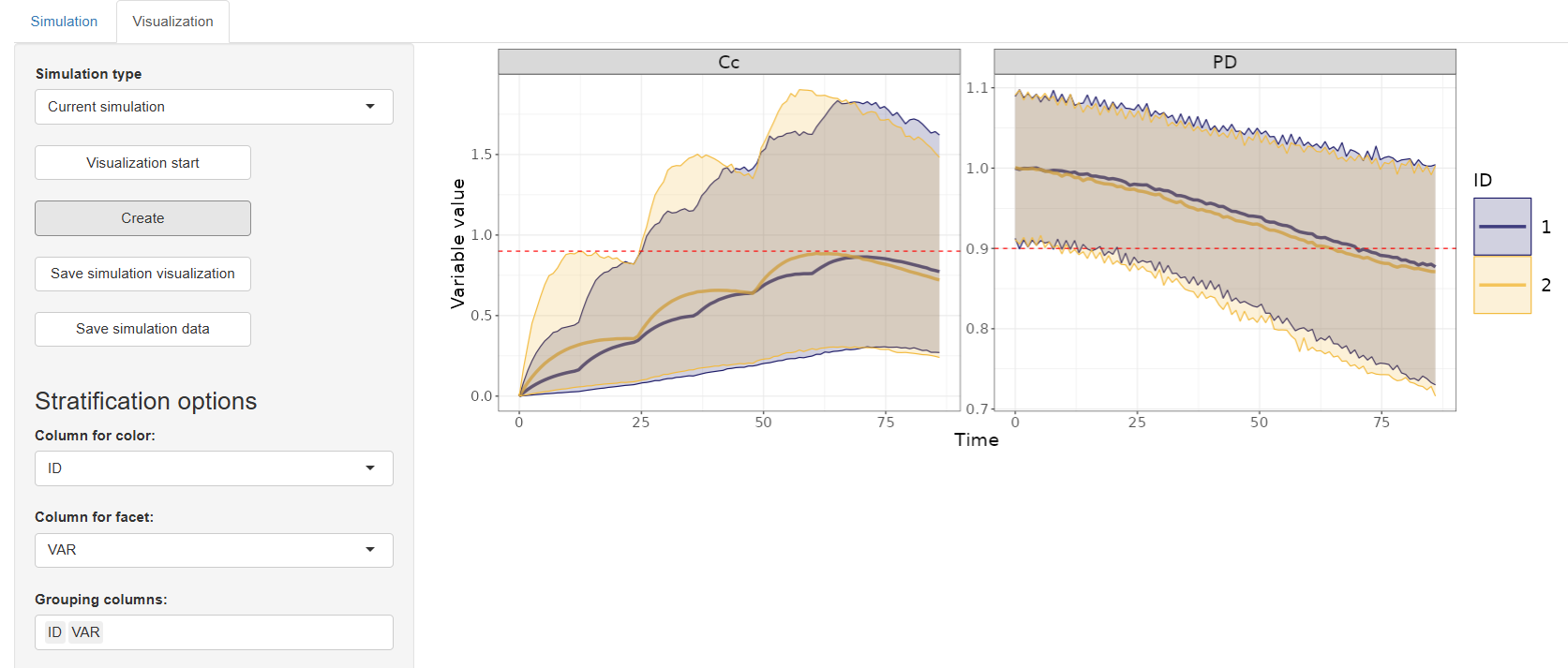
The Visualization tab lets you explore simulation results interactively or load results from a previous run. All plotting and export tools are accessed from the left-hand settings panel.
Work in this tab begins by choosing a Simulation type:
- Current simulation – Displays the results produced by the configuration set in the Simulation tab.
- New simulation – Uploads a
.csvfile containing results from an earlier simulation for standalone visualization.- CSV requirements (New simulation): The file must contain the following columns:
ID– scenario or subject identifiersim.id– replicate index (e.g., population, subject, or residual-error draw)TIME– simulation time pointsVAR– name of the simulated variables or metricVALUE– simulated value at each time point
- CSV requirements (New simulation): The file must contain the following columns:
After selecting the desired source, click  .
The rest of the control panel becomes active.
.
The rest of the control panel becomes active.
Core Actions
-
 generates the plot using the current settings. The first time you press Create, a default configuration is applied automatically..
 -
 exports the current plot to the working directory defined in the Task section.
 -
 writes the underlying numerical results to a
 .csvfile in the same working directory.
Configuration Blocks
After clicking , the configuration panel appears on the left side of the interface. It is divided into three main blocks: Stratification options, Display options, and Plot options. Each block contains specific tools for customizing how simulation results are visualized.
1. Stratification Options
Use this section to organize and differentiate the data shown in the plot:
-
Column for color – Select a variable that determines the color of the plot lines.
-
Column for facet – Splits the output into multiple subplots, each for a different value of the selected variable.
-
Grouping columns – Specify one or more variables to group simulation results for summarization or visual distinction.
-
Column for linetype – Assigns different line styles based on the values of the selected variable.
-
Plotted scenarios (ID) – Choose which scenario IDs (as defined in the Simulation tab) to include in the plot.
-
Plotted outputs – Select which outputs to visualize. If no outputs were chosen during simulation setup, all available outputs will be listed.
-
Aggregate by ID – When enabled, displays the aggregated output across selected IDs. Currently, only mean aggregation is available.
2. Display Options
This section provides options to enhance the visual information shown in the plot:
-
Add legend – Includes a legend for interpreting colors, line types, and groups.
-
Measure of central tendency – Choose between mean and median as the primary statistic. If mean is selected, you can also show prediction intervals of:
- 50%, 90%, 95%, or 99%
-
Add validation data – Enables comparison with observed or reference data. Two options appear when enabled:
-
Validation data source – Choose between:
- Event table data (based on simulation input),
- New data (upload a file).
-
Add error bars – Show error bars on the validation data points, if available.
-
3. Plot Options
Use these tools to customize the appearance and add analytical features to the plot:
-
Axis labels – Set custom labels for the X and Y axes.
-
Log scale – Apply logarithmic scaling to the X and/or Y axes.
-
Axis limits – Manually adjust the range for each axis.
-
Add vertical line – Insert a vertical reference line at specified time points.
-
Add horizontal line – Insert a horizontal reference line (e.g., threshold levels).
The result of your configured settings is the simulation plot displayed in the main panel. It reflects all the selected parameters and visual preferences defined in configuration blocks.
Tables Generation
Below the plot, several tools are available for generating detailed tables based on your simulation results. Each tool complements the graphical output with structured data for deeper analysis.
Responders table
Clicking the  button generates the Responders Table, which provides insights into how simulated outputs perform relative to a defined threshold (set in the "Add horizontal line" option under Plot Options).
This table displays:
- Results grouped by
ID- scenario ID andVAR- output variable . - The percentage of values below and above the threshold.
This is especially useful for quantifying responder rates or evaluating cutoff-based metrics.

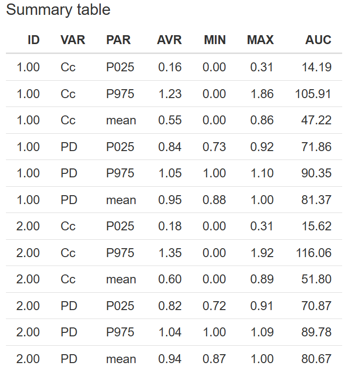
Summary Table
Clicking the  button produces the Summary Table, which summarizes key statistics for each simulated output and scenario.
Included in the table:
- Results grouped by
ID- scenario ID andVAR- output variable . PARcolumn reflects the levels associated with the selected measure of central tendency and interval defined in the Display options configuration block.MIN- minimum andMAX- maximumAUC(Area Under the Curve)
This table is helpful for assessing distributional properties and comparative analysis across scenarios.
Dosing Table
Clicking the  button displays the Dosing Table, which outlines the dosing structure defined in each simulation scenario.
It reflects the dosing inputs as set in the Simulation Scenarios subsection of the Simulation tab and includes columns such as:
ID,TIME,CMT,ADDL,IIand depending on simulaty type:AMTfor Time profilesMinDose / MaxDosefor Dose-response
- Plus any additional columns defined by the user
This table is useful for reviewing or exporting the dosing schedule associated with each scenario.