Model diagnostics
The purpose of this section is to diagnose the model with VPC plot (Visual Predictive Check plot), Covariate sensitivity plot and Table of model odds ratios.
Navigation
1 Model selection
The Model selection tab is used to choose the model for diagnostics and to add information about the covariates.
By clicking the  button, a file with the final models is loaded from the working directory. This file is generated in the Covariate search section. Make sure that the file with models has been saved on that tab, otherwise notification “Project folder is empty” will appear.
Now, a model should be selected by response from the drop-down list 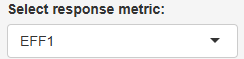 . Each response corresponds to one model.
Next, click  .
.
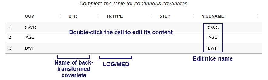
Before running diagnostics, additional information about covariates can be added, such as user-friendly names for plot labels or rescaling of model parameters. This information can be entered into the tables. To edit a cell, double-click it with the left mouse button.
1.1. Table of continuous covariates
Note that in the model transformed covariates can be used. Two types of transformed covariates are available:
-
Log-transformed
-
Median-centered
A median-centered covariate is a continuous covariate that has been transformed by subtracting its median value from each individual value. This results in a covariate whose median is zero, while the distribution and range of values remain the same (only shifted).
The Table of continuous covariates contains the following columns:
-
COV (“Covariate”) – automatically filled in from the model file. The first row corresponds to the exposure metric. The following rows contain the names of model continuous covariates.
-
BTR (“Back Transformed”) – contain the name of the corresponding untransformed covariate from the dataset, if the covariate listed in the COV column is transformed. Only filled in for transformed covariates. Example: If the COV column contains
LOGCAVG, which is obtained by log-transforming the values in theCAVGcolumn, then BTR should be set toCAVG. If the COV column containsMEDBWT("Median-centered Body Weight"), which is theBWT("Body Weight") covariate transformed by subtracting its median value from each observation, then BTR should be set toBWT. -
TRTYPE (“Transformation Type”) – two options are available:
LOG– for log-transformed covariates andMED– for median-centered covariates. Only filled in for transformed covariates. -
STEP – fill in to change the scale of odds-ratio. Odds-ratio will be calculated per STEP units of continuous covariate. By default odds-ratio is calculated per one unit of continuous covariate.
-
NICENAME – add a user-friendly name for covariate that will appear in plot labels and table
1.2. Table of categorical covariates
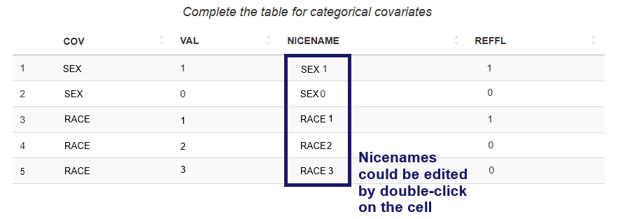
The Table of categorical covariates contains the following columns:
-
COV (“Covariate”) – contains the names of model categorical covariates. Automatically filled in from the model file.
-
VAL (“Value”) - contains numeric codes of categories from the dataset. Filled in automatically.
-
NICENAME - one can add a user-friendly name for the category that will appear in plot labels and table.
-
REFFL ("Reference Flag") - value
1indicates the reference category, while0corresponds to the other categories. Filled in automatically.
2. VPC plot
VPC plot is used to evaluate the fit and predictive performance of a logistic regression model relating drug exposure to the probability of response. It visualizes the model-predicted curve alongside empirical summaries of observed responses.
2.1. VPC plot description
A VPC plot example is shown in Figure 1.
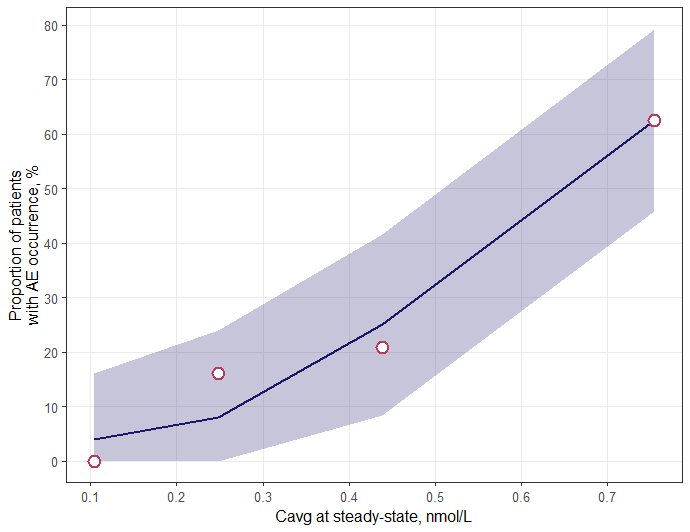
- X-axis: Exposure
- Y-axis: Predicted probability of response (in percent)
- Line: Median predicted probability curve from the model
- Shaded Area: Confidence Interval
- Points: Median observed response probability within each quantile of exposure
2.2. Visualization options
On the sidebar panel the following parameters can be changed:
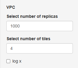
Number of replicas - number of simulated datasets generated using the model to estimate prediction intervals and assess the model's predictive performance.
Number of tiles - number of quartiles of exposure.
log x - add log-transformation of x-scale.
2.3. Running diagnostics
Click  button to start the analysis.
Click  to save the VPC plot. The results will be saved to the folder “Model diagnostics” in the working directory.
3. Sensitivity plot/Odds ratios table
3.1 Covariate sensitivity plot
The Covariate sensitivity plot is used to explore how covariates (both continuous and categorical) impact the odds of response across the range of drug exposure. Main purposes of this plot are to assess the sensitivity of predicted odds to changes in key covariates across the exposure range and to visualize whether covariate effects are constant, increasing, or decreasing with exposure.
A covariate sensitivity plot example is shown in Figure 2.
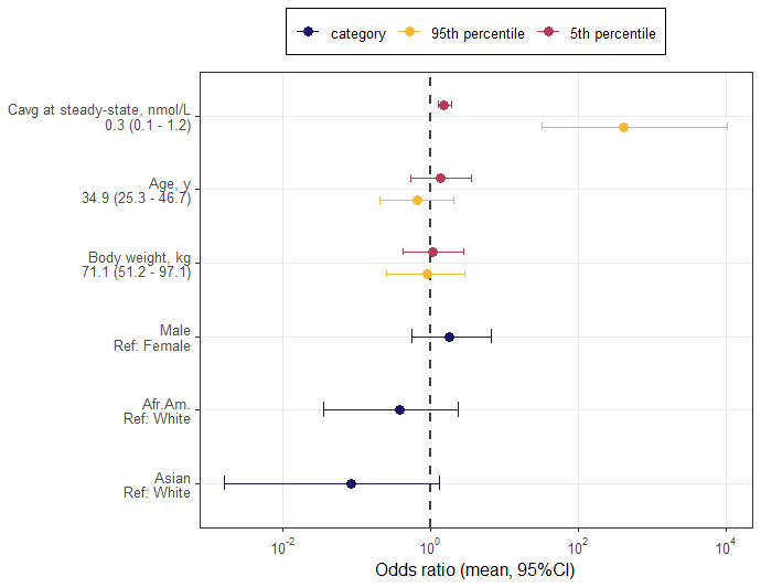
Plot description
- X-axis: Odds ratios — representing the effect of each covariate on the probability of response
- Y-axis: continuous and categorical covariates.
- Points: Estimated odds ratios for each covariate at different exposure levels
- Error Bars: Confidence intervals for the odds ratios
3.2. Visualization options
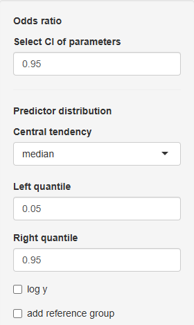
On the sidebar panel the some parameters can be changed:
Select CI of parameters - select confidence interval for odds ratio values (e.g. value \(0.95\) means \(95 \% \) confidence interval).
The following fields refer to Predictor distribution:
Central tendency – used for transformed continuous covariates. Specify median for covariates centered on the median, and mean for those centered on the mean.
Sensitivity analysis for continuous covariates is performed using the extreme quantiles of the covariate (e.g., \(0.05\) and \(0.95\) by default). On the plot, two points are shown for each continuous covariate, corresponding to the left quantile and right quantile.
Left quantile - left quantile value of continuous predictor.
Right quantile - right quantile value of continuous predictor.
log y - log-transformation of y-scale
add reference group
3.3. Table of odds ratios
Table of odds ratios presents the results of a logistic regression analysis, showing the estimated effects of exposure and covariates on the outcome, including regression coefficients, p-values, and odds ratios with confidence intervals for both unit-based and user-defined changes.
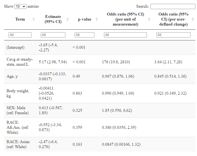
Table represents numerical values of odds ratios and contains the following columns:
Term - names of the model terms (predictors). This includes the intercept, continuous covariates (e.g., age, weight), and categorical variables (e.g. sex, race) with their reference categories.
Estimate (CI) - estimated regression coefficient and its confidence interval (CI) from the logistic regression model. This value represents the change in the log-odds of the response per unit increase in the predictor.
p-value - statistical significance of the predictor. A small p-value (typically \( < 0.05\)) suggests that the predictor has a statistically significant effect on the response.
Odds ratio (CI) (per unit of measurement) - odds ratio and its CI for a one-unit increase in the predictor (e.g., 1 year for age, 1 kg for weight). For categorical variables, it represents the odds ratio relative to the reference category.
Odds ratio (CI) (per user-defined change) - odds ratio and its CI based on a user-specified change in the predictor value. For example, this might be a 10-year change in age or a defined change in drug concentration. This column allows users to interpret effect sizes more meaningfully in the context of practical changes.
3.4. Running diagnostics
Click button to start the analysis.
Click  to save the plot and table. The results will be saved to the folder “Model diagnostics” in the working directory.