Creating a dataset for exposure-response analysis
On this page, you can create your own dataset for ER analysis.
1: Upload PK and Response data
First, navigate to the "Upload PK and Response data" tab.
1.1: Select the Working Directory
Here, you need to select the working directory by pressing  button. Working directory containing your project, which should include:
- The PK model (ModFile.txt)
- The dataset used for parameter fitting (DataTrans.csv)
- The Results folder with individual parameter values (Results/indiv_parameters.csv)
Your dataset should include the following columns:
ID- subject ID, numericAMT- dosage of the drug, numeric
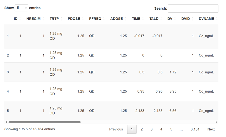
Once you select the working directory, the dataset will appear in the right panel, figure 1.
Initialize your PK data by pressing
 button.
After press button, if there are no necessary files or directors, you will see a notification in the lower right corner clarifying which file was not found.
1.2: Select the Exposure Data File
Next, select the file containing exposure data by pressing  button..
Once selected, the dataset will appear in the right panel, figure 2.
button..
Once selected, the dataset will appear in the right panel, figure 2.
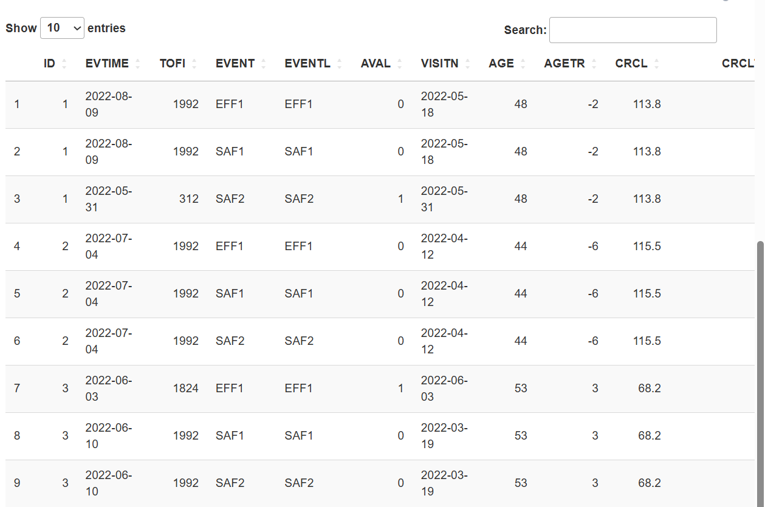
You should then specify which columns in your file represent:
Name of ID column- subject ID, numericName of TOFI column- the period of time from the moment of the first dosage to the first event, numericName of endpoint column- any type of dataName of response analise value column- for binary - 0 ot 1, numericName of nominal dosing column- for example: QD, QW, BID etc, any type of dataName of nominal frequency column- any type of data.Select covariate columns- сhoose the covarians with whom you will work further, any type of data
All of the above stakes, except for the covariat, will appear to be a recreational part of Response dataset.
We also recommend adding the EFFFL and SAFFL columns to your dataset. These columns should contain 1 for records corresponding to the respective endpoint type (efficacy or safety), and 0 otherwise. While these columns are not required, they allow you to save exposure–response datasets separately for each endpoint type.
After completing, initialize your response data by pressing  button.
2: Exposure-response dataset generation
Now that all required data is loaded, go to the ER dataset generation tab.
2.1: Choose the time intervals for simulation
In this section, you can run simulations over different time intervals to calculate exposure parameters. Select one or more time intervals for your ER dataset using the dropdown list Choose variables:.
Multiple simulations can be selected simultaneously.
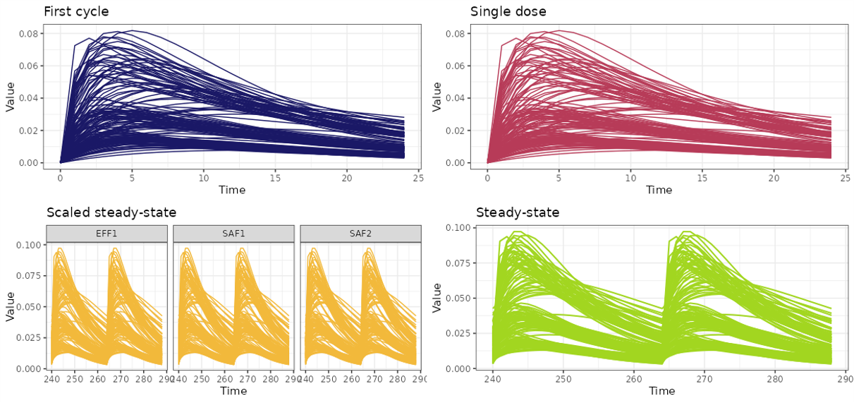
Time intervals explained:
First cycle- the time interval from the first dosing event to the end of the first cycle, based on the nominal dosing regimen.Single dose- the time interval from the first dosing event to the end of the first cycle, assuming only a single dose is administered.Scaled steady-state- the time interval equal to the length of one treatment cycle, starting from the time point at which the PK profile reaches steady-state. The dose used in the simulation is the average dose calculated over the period from the first dose up to the time of first incidence (TOFI).Steady-state- the time interval equal to the length of one treatment cycle, starting from the time point at which the PK profile reaches steady-state. The simulation uses the nominal dosing regimen.
For all simulations, you need to define Cycle duration, which should be entered in the Enter a Cycle duration field.
For Scaled steady-state and Steady-state simulations, you also need to define "Steady state cycle", which should be entered in the Enter a Steady state cycle field.
You also need to choose a variable of the model from the dropdown list Simulation output, for which you will make the simulations. In the dropdown list you will see all model variables that were taken from the control file.
Once all fields are filled and the simulation types are selected, start the simulations by pressing  button.
After completion, the simulation results will be visualized in the right panel.
button.
After completion, the simulation results will be visualized in the right panel.
You can save the generated plots to the Results folder in your working directory by pressing  button. The file will be saved as
 Results/exposure_simulation.png.
2.2: Select Exposure parameters
Now we can calculate Exposure-Response based on data obtained after simulations for this you should select the exposure parameters needed for further analysis.
Metrics can be selected from the dropdown list Choose exposure metrics:, with the option to choose multiple metrics at once.
Exposure parameters Explained:
- Cmax - the maximum concentration of the drug
- Cmin - the minimum concentration of the drug
- Cavr - the average concentration of the drug
- AUC - the square under the drug pharmacokinetics curve
After chosed exposure metrics, start the estimation by pressing  button.
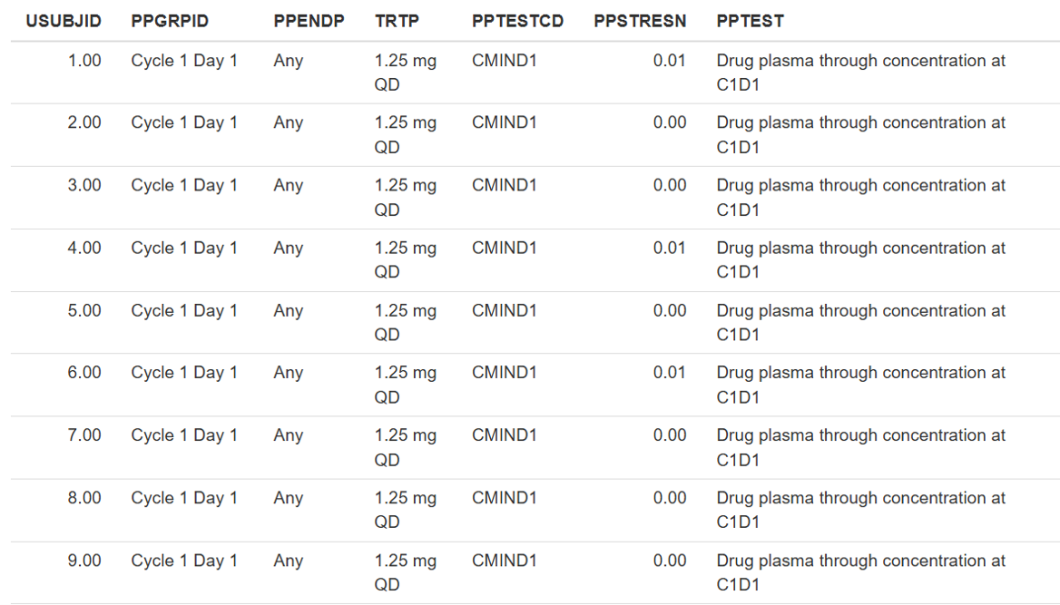
The final table, exposure data will appear in the right panel.
2.3: Save results
To save the SIMPC and SIMPP datasets, click the  button. The files will be saved in the same folder as your exposure dataset, as
 simpc.csv and simpp.csv, respectively.
To generate and save the exposure–response dataset, select which endpoints you want to include from the dropdown menu ADER dataset type: all Efficacy or all Safety endpoints. Then click the  button. The data will be saved in the same folder as your exposure dataset, as
 adereff.csv or adersaf.csv, respectively.
If your exposure dataset does not contain the EFFFL and SAFFL flags, the exposure–response dataset will include all endpoints and be saved as adereff.csv in the same folder.
After the exposure–response file is generated, a notification will appear in the bottom-right corner indicating which endpoints were included (Figure 5).
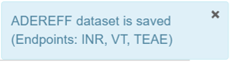
Figure 5. Expample of notification. In adereff.csv saved exposure–response data for "INR", "VT", "TEAE" endpoints.